Fitting distributions using primarycensored and cmdstan
Source:vignettes/fitting-dists-with-stan.Rmd
fitting-dists-with-stan.Rmd1 Introduction
1.1 What are we going to do in this vignette
In this vignette, we’ll demonstrate how to use primarycensored in conjunction with Stan for Bayesian inference of epidemiological delay distributions. We’ll cover the following key points:
- Simulating censored delay distribution data
- Fitting a naive model using cmdstan
- Evaluating the naive model’s performance
- Fitting an improved model using
primarycensoredfunctionality - Fitting the same model using
primarycensored’s built in cmdstan model. - Comparing the
primarycensoredmodel’s performance to the naive model
1.2 What you will learn
By the end of this vignette, you will be able to:
- Understand the bias introduced by ignoring primary censoring and truncation when fitting delay distributions
- Use
pcd_cmdstan_model()andpcd_as_stan_data()to fit distributions that properly account for primary censoring, secondary censoring, and truncation - Understand when Bayesian fitting with Stan is appropriate versus MLE approaches with fitdistrplus
1.3 What might I need to know before starting
This vignette builds on the concepts introduced in the Getting started with primarycensored vignette and assumes familiarity with using Stan tools as covered in the How to use primarycensored with Stan vignette.
2 Simulating censored and truncated delay distribution data
We’ll start by simulating some censored and truncated delay distribution data. We’ll use the rprimarycensored function (actually we will use the rpcens alias for brevity).
set.seed(123) # For reproducibility

# Define the number of samples to generate
n <- 2000

# Define the true distribution parameters
meanlog <- 1.5
sdlog <- 0.75

# Generate varying pwindow, swindow, and obs_time lengths
pwindows <- sample.int(2, n, replace = TRUE)
swindows <- sample.int(2, n, replace = TRUE)
obs_times <- sample(8:10, n, replace = TRUE)

# Function to generate a single sample
generate_sample <- function(pwindow, swindow, obs_time) {
  rpcens(
    1, rlnorm,
    meanlog = meanlog, sdlog = sdlog,
    pwindow = pwindow, swindow = swindow, D = obs_time
  )
}

# Generate samples
samples <- mapply(generate_sample, pwindows, swindows, obs_times)

# Create initial data frame
delay_data <- data.frame(
  pwindow = pwindows,
  obs_time = obs_times,
  observed_delay = samples, # this is the observed i.e. censored delay
  observed_delay_upper = samples + swindows # The upper bound of the delay3
  # (i.e. the true delay is between the observed and the upper bound)
) |>
  mutate(
    observed_delay_upper = pmin(obs_time, observed_delay_upper)
  )

head(delay_data)
## pwindow obs_time observed_delay observed_delay_upper
## 1 1 9 3 4
## 2 1 9 4 5
## 3 1 8 6 7
## 4 2 10 6 8
## 5 1 10 8 10
## 6 2 8 4 5
# Aggregate to unique combinations and count occurrences
delay_counts <- delay_data |>
  summarise(
    n = n(),
    .by = c(pwindow, obs_time, observed_delay, observed_delay_upper)
  )

head(delay_counts)
## pwindow obs_time observed_delay observed_delay_upper n
## 1 1 9 3 4 37
## 2 1 9 4 5 31
## 3 1 8 6 7 16
## 4 2 10 6 8 26
## 5 1 10 8 10 22
## 6 2 8 4 5 43
# Compare the samples with and without secondary event censoring to the true
# distribution
# Calculate empirical CDF
empirical_cdf <- ecdf(samples)

# Create a sequence of x values for the theoretical CDF
x_seq <- seq(min(samples), max(samples), length.out = 100)

# Calculate theoretical CDF
theoretical_cdf <- plnorm(x_seq, meanlog = meanlog, sdlog = sdlog)

# Create a long format data frame for plotting
cdf_data <- data.frame(
  x = rep(x_seq, 2),
  probability = c(empirical_cdf(x_seq), theoretical_cdf),
  type = rep(c("Observed", "Theoretical"), each = length(x_seq)),
  stringsAsFactors = FALSE
)

# Plot
ggplot(cdf_data, aes(x = x, y = probability, color = type)) +
  geom_step(linewidth = 1) +
  scale_color_manual(
    values = c(Observed = "#4292C6", Theoretical = "#252525")
  ) +
  geom_vline(
    aes(xintercept = mean(samples), color = "Observed"),
    linetype = "dashed", linewidth = 1
  ) +
  geom_vline(
    aes(xintercept = exp(meanlog + sdlog^2 / 2), color = "Theoretical"),
    linetype = "dashed", linewidth = 1
  ) +
  labs(
    title = "Comparison of Observed vs Theoretical CDF",
    x = "Delay",
    y = "Cumulative Probability",
    color = "CDF Type"
  ) +
  theme_minimal() +
  theme(
    panel.grid.minor = element_blank(),
    plot.title = element_text(hjust = 0.5),
    legend.position = "bottom"
  )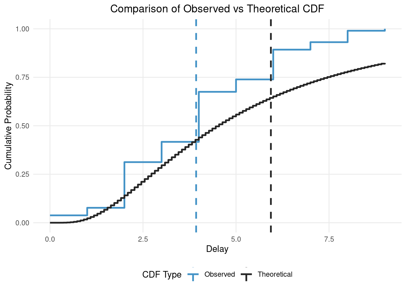
In this figure you can see the impact of truncation and censoring as the observed distribution has a much lower mean (the vertical dashed blue line) than the true/theoretical distribution (the vertical dashed black line). Our modelling aim is to recover the true parameters of the theoretical distribution from the observed distribution (i.e. recover the black lines from the blue lines).
We’ve aggregated the data to unique combinations of pwindow, swindow, and obs_time and counted the number of occurrences of each observed_delay for each combination. This is the data we will use to fit our model.
3 Fitting a naive model using cmdstan
We’ll start by fitting a naive model using cmdstan. We’ll use the cmdstanr package to interface with cmdstan. We define the model in a string and then write it to a file as in the How to use primarycensored with Stan vignette.
writeLines(
  "data {
    int<lower=0> N;  // number of observations
    vector[N] y;     // observed delays
    vector[N] n;     // number of occurrences for each delay
  }
  parameters {
    real mu;
    real<lower=0> sigma;
  }
  model {
    // Priors
    mu ~ normal(1, 1);
    sigma ~ normal(0.5, 1);

    // Likelihood
    target += n .* lognormal_lpdf(y | mu, sigma);
  }",
  con = file.path(tempdir(), "naive_lognormal.stan")
)
Now let’s compile the model
naive_model <- cmdstan_model(file.path(tempdir(), "naive_lognormal.stan"))and now let’s fit the compiled model.
naive_fit <- naive_model$sample(
  data = list(
    # Add a small constant to avoid log(0)
    y = delay_counts$observed_delay + 1e-6,
    n = delay_counts$n,
    N = nrow(delay_counts)
  ),
  chains = 4,
  parallel_chains = 4,
  refresh = ifelse(interactive(), 50, 0),
  show_messages = interactive()
)
naive_fit
## variable mean median sd mad q5 q95 rhat ess_bulk
## lp__ -381721.38 -381721.10 0.99 0.76 -381723.44 -381720.42 1.00 1817
## mu -0.60 -0.60 0.01 0.01 -0.62 -0.58 1.00 1601
## sigma 5.10 5.10 0.01 0.01 5.08 5.11 1.00 3935
## ess_tail
## 2101
## 1882
## 2752You may see a warning that NAs introduced by coercion this can be ignored as it is an artefact of this simple example model.
We see that the model has converged and the diagnostics look good. However, just from the model posterior summary we see that we might not be very happy with the fit. mu is smaller than the target 1.5 and sigma is larger than the target 0.75. Note that the mu and sigma parameters are the meanlog and sdlog parameters of the lognormal distribution.
4 Fitting an improved model using primarycensored
We’ll now fit an improved model using the primarycensored package. The main improvement is that we will use the primarycensored_lpdf function to fit the model. This is the Stan version of the pcens() function and adjusts for the primary and secondary censoring windows as well as the truncation. We encode that our primary distribution is a lognormal distribution by passing 1 as the dist_id parameter and that our primary event distribution is uniform by passing 1 as the primary_id parameter. See the Stan documentation for more details on the primarycensored_lpdf function.
writeLines(
  "
  functions {
    #include primarycensored.stan
    // These functions are required for the primarycensored_lpdf function
    #include primarycensored_ode.stan
    #include primarycensored_analytical_cdf.stan
    #include expgrowth.stan
  }
  data {
    int<lower=0> N;  // number of observations
    array[N] int<lower=0> y;     // observed delays
    array[N] int<lower=0> y_upper;     // observed delays upper bound
    array[N] int<lower=0> n;     // number of occurrences for each delay
    array[N] int<lower=0> pwindow; // primary censoring window
    array[N] int<lower=0> D; // maximum delay
  }
  transformed data {
    array[0] real primary_params;
  }
  parameters {
    real mu;
    real<lower=0> sigma;
  }
  model {
    // Priors
    mu ~ normal(1, 1);
    sigma ~ normal(0.5, 0.5);

    // Likelihood
    for (i in 1:N) {
      target += n[i] * primarycensored_lpmf(
        y[i] | 1, {mu, sigma},
        pwindow[i], y_upper[i], 0, D[i],
        1, primary_params
      );
    }
  }",
  con = file.path(tempdir(), "primarycensored_lognormal.stan")
)
Now let’s compile the model
primarycensored_model <- cmdstan_model(
  file.path(tempdir(), "primarycensored_lognormal.stan"),
  include_paths = pcd_stan_path()
)
Now let’s fit the compiled model.
primarycensored_fit <- primarycensored_model$sample(
  data = list(
    y = delay_counts$observed_delay,
    y_upper = delay_counts$observed_delay_upper,
    n = delay_counts$n,
    pwindow = delay_counts$pwindow,
    D = delay_counts$obs_time,
    N = nrow(delay_counts)
  ),
  chains = 4,
  parallel_chains = 4,
  refresh = ifelse(interactive(), 50, 0),
  show_messages = interactive()
)
primarycensored_fit
## variable mean median sd mad q5 q95 rhat ess_bulk ess_tail
## lp__ -3422.74 -3422.44 0.99 0.71 -3424.71 -3421.79 1.00 1369 1861
## mu 1.55 1.54 0.05 0.05 1.48 1.62 1.00 1122 1213
## sigma 0.78 0.78 0.03 0.03 0.73 0.84 1.00 1063 1227We see that the model has converged and the diagnostics look good. We also see that the posterior means are very near the true parameters and the 90% credible intervals include the true parameters.
5 Using pcd_cmdstan_model() for a more efficient approach
While the previous approach works well, primarycensored provides a more efficient and convenient model which we can compile using pcd_cmdstan_model(). This approach not only saves time in model specification but also leverages within chain parallelisation to make best use of your machine’s resources. Alongside this we also supply a convenience function pcd_as_stan_data() to convert our data into a format that can be used to fit the model and supply priors, bounds, and other settings.
Let’s use this function to fit our data:
# Compile the model with multithreading support
pcd_model <- pcd_cmdstan_model(cpp_options = list(stan_threads = TRUE))

pcd_data <- pcd_as_stan_data(
  delay_counts,
  delay = "observed_delay",
  delay_upper = "observed_delay_upper",
  relative_obs_time = "obs_time",
  dist_id = pcd_stan_dist_id("lognormal", "delay"),
  primary_id = pcd_stan_dist_id("uniform", "primary"),
  param_bounds = list(lower = c(-Inf, 0), upper = c(Inf, Inf)),
  primary_param_bounds = list(lower = numeric(0), upper = numeric(0)),
  priors = list(location = c(1, 0.5), scale = c(1, 0.5)),
  primary_priors = list(location = numeric(0), scale = numeric(0)),
  use_reduce_sum = TRUE # use within chain parallelisation
)

pcd_fit <- pcd_model$sample(
  data = pcd_data,
  chains = 4,
  parallel_chains = 2, # Run 2 chains in parallel
  threads_per_chain = 2, # Use 2 cores per chain
  refresh = ifelse(interactive(), 50, 0),
  show_messages = interactive()
)

pcd_fit
## variable mean median sd mad q5 q95 rhat ess_bulk ess_tail
## lp__ -3422.76 -3422.45 1.03 0.73 -3424.85 -3421.79 1.01 1361 1825
## params[1] 1.54 1.54 0.05 0.04 1.47 1.63 1.01 1220 1237
## params[2] 0.78 0.78 0.03 0.03 0.73 0.83 1.01 1250 1381In this model we have a generic params vector that contains the parameters for the delay distribution. In this case these are mu and sigma from the last example (i.e. the meanlog and sdlog parameters of the lognormal distribution). We also have a primary_params vector that contains the parameters for the primary distribution. In this case this is empty as we are using a uniform distribution.
We see again that the model has converged and the diagnostics look good. We also see that the posterior means are very near the true parameters and the 90% credible intervals include the true parameters as with the manually written model. Note that we have set parallel_chains = 2 and threads_per_chain = 2 to demonstrate within chain parallelisation. Usually however you would want to use parallel_chains = <number of chains> and then use the remainder of the available cores for within chain parallelisation by setting threads_per_chain = <remaining cores / number of chains> to ensure that you make best use of your machine’s resources.
5.1 Summary
In this vignette we have shown how to fit a delay distribution using primarycensored in conjunction with cmdstan. The key takeaways are:
-
Use
pcd_cmdstan_model()andpcd_as_stan_data(): This is the recommended approach for most users. It handles all the complexity of primary censoring, secondary censoring, and truncation automatically, and supports within-chain parallelisation. -
Specify distributions by ID: Use
pcd_stan_dist_id()to get the correct distribution identifier (e.g.,"lognormal","gamma","weibull"). - Ignoring censoring causes bias: The naive model that ignores primary censoring and truncation substantially underestimates the true distribution parameters.
For a faster MLE-based approach that doesn’t require Stan, see the vignette("fitting-dists-with-fitdistrplus") vignette. For fitting delay distributions that can take negative values (e.g. logistic-distributed serial intervals), see the vignette("fitting-negative-support") vignette. For more flexible delay distribution fitting, see the epidist package (which uses primarycensored under the hood).
5.2 How you might adapt this vignette
This vignette uses simulated data, but you can adapt it for your own work:
-
Replace simulation with real data: Swap out the simulated
delay_datawith your own observations of delays between primary and secondary events -
Change the distribution: Replace
"lognormal"with other distributions like"gamma"or"weibull"usingpcd_stan_dist_id() -
Vary the censoring windows: Adjust
pwindowvalues to match your data’s actual primary censoring intervals -
Handle different truncation times: Use varying values in the
obs_timecolumn if your observations have different maximum observable delays -
Add lower truncation: If you need to exclude delays below a minimum value (e.g., for generation intervals where day 0 is excluded in renewal models), add a
start_relative_obs_timecolumn to your data specifying the lower truncation point L for each observation. Values may be any finite real number or-Inf(the default when the column is absent), mirroring the R-sidepprimarycensored()interface. -
Modify priors: Adjust the
priorsargument inpcd_as_stan_data()to reflect your prior knowledge about the distribution parameters