Fitting distributions using primarycensored and fitdistrplus

1 Introduction

1.1 What are we going to do in this vignette

In this vignette, we’ll demonstrate how to use primarycensored in conjunction with fitdistrplus for fitting distributions. We’ll cover the following key points:

Simulating censored delay distribution data
Fitting a naive model using fitdistrplus
Evaluating the naive model’s performance
Fitting an improved model using primarycensored functionality
Comparing the primarycensored model’s performance to the naive model

1.2 What might I need to know before starting

This vignette assumes some familiarity with the fitdistrplus package. If you are not familiar with it then you might want to start with the Introduction to fitdistrplus vignette.

1.3 How does this vignette differ from fitting distributions with Stan vignette

This vignette is similar to the vignette("fitting-dists-with-stan") vignette in that it shows how to fit a distribution using primarycensored. However, here we use maximum likelihood estimation (MLE) to fit the distribution, rather than MCMC. In some settings this may result in a faster fit, but in other settings especially when the data is complex, MCMC may be more reliable. The major benefit of the fitdistrplus approach is that we don’t need to install additional software (Stan) to fit the distribution. Note that rather than returning credible intervals, the fitdistrplus package returns standard errors and confidence intervals.

1.4 Packages used in this vignette

Alongside the primarycensored package we will use the fitdistrplus package for fitting distributions. We will also use the ggplot2 package for plotting and dplyr for data manipulation.

library(primarycensored)
library(fitdistrplus)
library(ggplot2)
library(dplyr)

2 Simulating censored and truncated delay distribution data

We’ll start by simulating some censored and truncated delay distribution data. We’ll use the rprimarycensored function (actually we will use the rpcens alias for brevity).

set.seed(123) # For reproducibility

# Define the number of samples to generate
n <- 1000

# Define the true distribution parameters
shape <- 1.77 # This gives a mean of 4 and sd of 3 for a gamma distribution
rate <- 0.44

# Generate fixed pwindow, swindow, and obs_time
pwindows <- rep(1, n)
swindows <- rep(1, n)
obs_times <- sample(8:10, n, replace = TRUE)

# Function to generate a single sample
generate_sample <- function(pwindow, swindow, obs_time) {
  rpcens(
    1, rgamma,
    shape = shape, rate = rate,
    pwindow = pwindow, swindow = swindow, D = obs_time
  )
}

# Generate samples
samples <- mapply(generate_sample, pwindows, swindows, obs_times)

# Create initial data frame
delay_data <- data.frame(
  delay = samples,
  delay_upper = samples + swindows,
  pwindow = pwindows,
  relative_obs_time = obs_times
)

head(delay_data)

##   delay delay_upper pwindow relative_obs_time
## 1     2           3       1                10
## 2     1           2       1                10
## 3     2           3       1                10
## 4     4           5       1                 9
## 5     3           4       1                10
## 6     4           5       1                 9

# Compare the samples with and without secondary censoring to the true
# distribution
# Calculate empirical CDF
empirical_cdf <- ecdf(samples)

# Create a sequence of x values for the theoretical CDF
x_seq <- seq(0, 10, length.out = 100)

# Calculate theoretical CDF
theoretical_cdf <- pgamma(x_seq, shape = shape, rate = rate)

# Create a long format data frame for plotting
cdf_data <- data.frame(
  x = rep(x_seq, 2),
  probability = c(empirical_cdf(x_seq), theoretical_cdf),
  type = rep(c("Observed", "Theoretical"), each = length(x_seq)),
  stringsAsFactors = FALSE
)

# Plot
ggplot(cdf_data, aes(x = x, y = probability, color = type)) +
  geom_step(linewidth = 1) +
  scale_color_manual(
    values = c(Observed = "#4292C6", Theoretical = "#252525")
  ) +
  geom_vline(
    aes(xintercept = mean(samples), color = "Observed"),
    linetype = "dashed", linewidth = 1
  ) +
  geom_vline(
    aes(xintercept = shape / rate, color = "Theoretical"),
    linetype = "dashed", linewidth = 1
  ) +
  labs(
    title = "Comparison of Observed vs Theoretical CDF",
    x = "Delay",
    y = "Cumulative Probability",
    color = "CDF Type"
  ) +
  theme_minimal() +
  theme(
    panel.grid.minor = element_blank(),
    plot.title = element_text(hjust = 0.5),
    legend.position = "bottom"
  ) +
  coord_cartesian(xlim = c(0, 10)) # Set x-axis limit to match truncation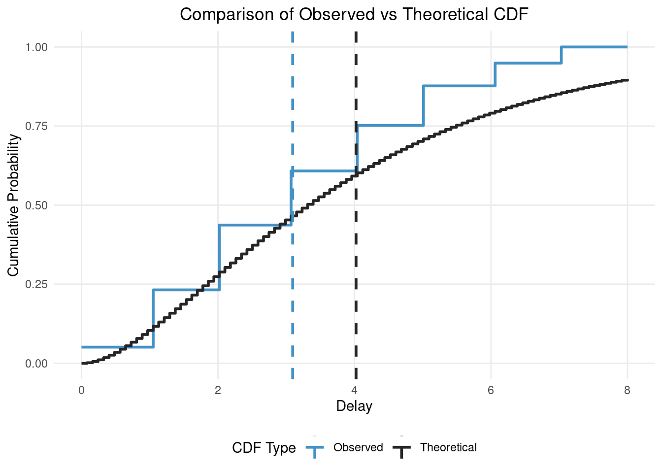

In this figure you can see the impact of truncation and censoring as the observed distribution has a much lower mean (the vertical dashed blue line) than the true/theoretical distribution (the vertical dashed black line). Our modelling aim is to recover the true parameters of the theoretical distribution from the observed distribution (i.e. recover the black lines from the blue lines).

3 Fitting a naive model using `fitdistrplus`

We first fit a naive model using the fitdistcens() function. This function is designed to handle secondary censored data but does not handle primary censoring or truncation without extension.

fit <- delay_data |>
  dplyr::select(left = delay, right = delay_upper) |>
  fitdistcens(
    distr = "gamma",
    start = list(shape = 1, rate = 1)
  )

summary(fit)

## Fitting of the distribution ' gamma ' By maximum likelihood on censored data 
## Parameters
##        estimate Std. Error
## shape 2.9607131 0.13487956
## rate  0.7788964 0.03808087
## Loglikelihood:  -2111.847   AIC:  4227.693   BIC:  4237.509 
## Correlation matrix:
##           shape      rate
## shape 1.0000000 0.9253887
## rate  0.9253887 1.0000000

We see that the naive model has fit poorly due to the primary censoring and right truncation in the data.

4 Fitting an improved model using `primarycensored` and `fitdistrplus`

We’ll now fit an improved model using the primarycensored package. To do this we need to define the custom distribution functions using the primarycensored package that are required by fitdistrplus. Rather than using fitdistcens we use fitdist because our functions are handling the censoring themselves. Note that in this custom implementation for simplicity we are filtering to use only data with the same obs_time rather than handling varying observation times. This means we’re using a subset of our simulated data for the estimation.

# Define custom distribution functions using primarycensored
# The try catch is required by fitdistrplus
dpcens_gamma <- function(x, shape, rate) {
  result <- tryCatch(
    {
      dprimarycensored(
        x, pgamma,
        shape = shape, rate = rate,
        pwindow = 1, swindow = 1, D = 8
      )
    },
    error = function(e) {
      rep(NaN, length(x))
    }
  )
  return(result)
}

ppcens_gamma <- function(q, shape, rate) {
  result <- tryCatch(
    {
      pprimarycensored(
        q, pgamma,
        shape = shape, rate = rate,
        dpwindow = 1, D = 8
      )
    },
    error = function(e) {
      rep(NaN, length(q))
    }
  )
  return(result)
}

# Fit the model using fitdistcens with custom gamma distribution
pcens_fit <- delay_data |>
  dplyr::filter(relative_obs_time == 8) |>
  dplyr::pull(delay) |>
  fitdist(
    distr = "pcens_gamma",
    start = list(shape = 1, rate = 1)
  )

summary(pcens_fit)

## Fitting of the distribution ' pcens_gamma ' by maximum likelihood 
## Parameters : 
##        estimate Std. Error
## shape 1.7522811 0.19551646
## rate  0.4734692 0.08187069
## Loglikelihood:  -639.2144   AIC:  1282.429   BIC:  1290.003 
## Correlation matrix:
##           shape      rate
## shape 1.0000000 0.9266603
## rate  0.9266603 1.0000000

We see good agreement between the true and estimated parameters but with higher standard errors due to using a subset of the data.

Rather than using fitdist() directly primarycensored provides a wrapper function fitdistdoublecens() that can be used to estimate double censored and truncated data. A bonus of this approach is we can specify our data using the fitdistcens left and right formulation and support mixed censoring intervals. Another bonus of this approach is that it supports a mixture of observation times so we can fit to all the available data rather than the subset we used in the custom implementation above.

# Using Stan-like interface but with fitdistrplus
fitdistdoublecens_fit <- fitdistdoublecens(
  delay_data,
  distr = "gamma",
  start = list(shape = 1, rate = 1),
  left = "delay",
  right = "delay_upper",
  pwindow = "pwindow",
  D = "relative_obs_time"
)

summary(fitdistdoublecens_fit)

## Fitting of the distribution ' pcens_dist ' by maximum likelihood 
## Parameters : 
##        estimate Std. Error
## shape 1.6863057 0.10294344
## rate  0.4213108 0.03945095
## Loglikelihood:  -2064.778   AIC:  4133.556   BIC:  4143.371 
## Correlation matrix:
##           shape      rate
## shape 1.0000000 0.9196305
## rate  0.9196305 1.0000000

4.1 Summary

In this vignette we have shown how to fit a distribution using primarycensored in conjunction with fitdistrplus both from scratch and using the fitdistdoublecens() function. We have also shown how to compare the performance of the primarycensored model to a naive model.

If interested in a more robust approach to fitting distributions see the vignette("fitting-dists-with-stan") vignette. If you are instead interested in fitting a delay distribution more flexibly see the epidist package (which uses primarycensored under the hood).

Sam Abbott